


Interpreting historic lake water phosphorus changes and catchment sources at Semer Water
Dr John Boyle, Dr Madeleine Moyle University of Liverpool (maddy.moyle@liverpool.ac.uk | jfb@liverpool.ac.uk)
Sediment core provided by: Richard Chiverrell & David Sear
[Image: The University of Liverpool logo is in the top right corner. The title and author information are contained within white rectangular borders against a dark blue background.]
Contents
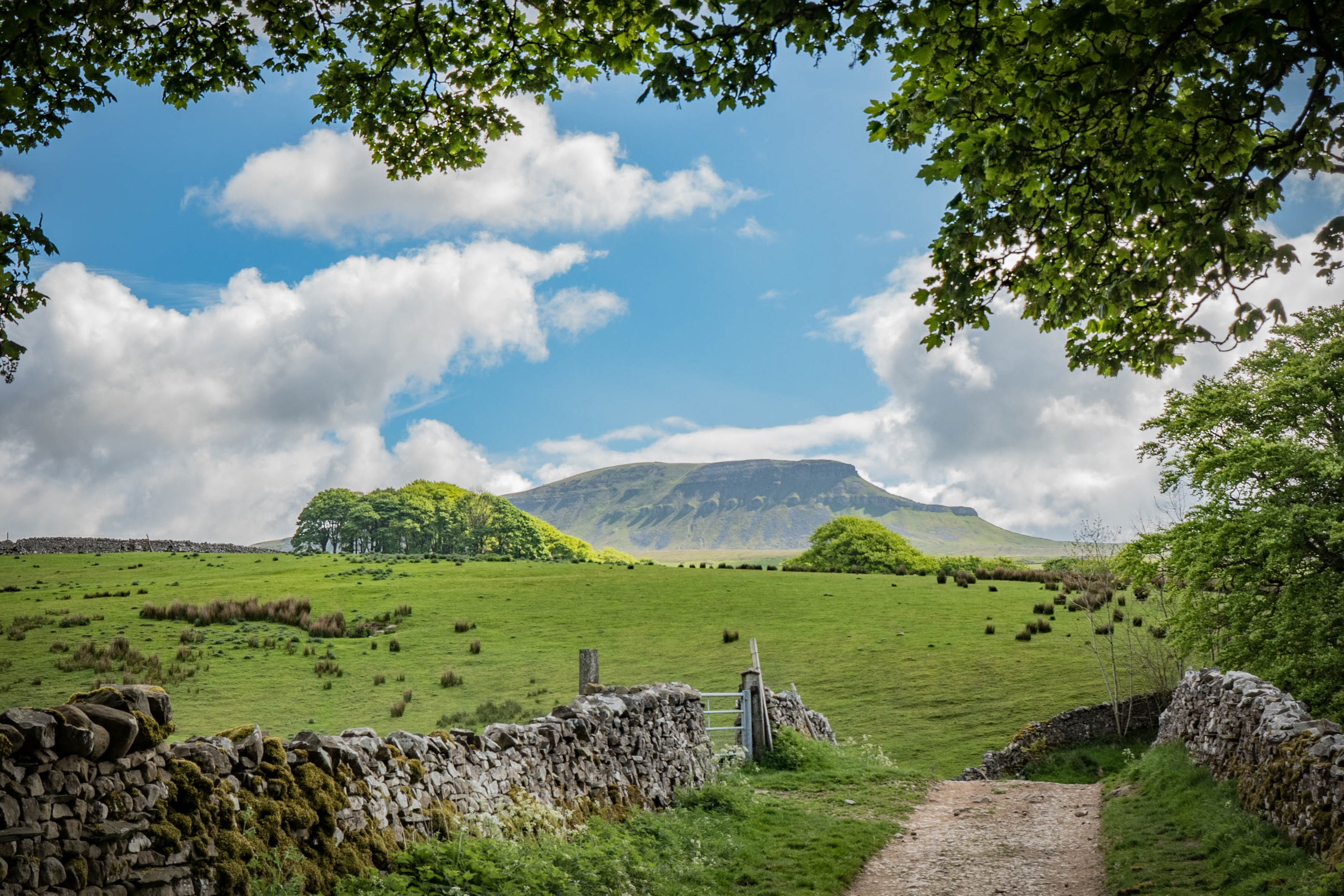
[Image: A photograph of Semer Water in a valley, surrounded by green hills, trees, and a stone wall in the foreground.]
- Using lake sediment record to examine historic phosphorus trends
- Modelling a phosphorus budget for Semer Water
- Determining phosphorus sources
About us
[Image: Four photographs showing researchers at work. One shows two people in an inflatable boat on a lake. Another shows a researcher sitting in a boat with a small dog wearing a yellow life jacket. A third shows a researcher holding a sample bottle and the dog. The fourth shows a man on a wooden pier pulling a long sediment core tube out of the water.]
Palaeolimnologist, Sedimentologist, Geochemist, Hydrologist, Limnologist, Geologist, Archaeologist, Field researcher, Lab researcher, Modeller
What do we do? We take sediment (mud) from the bottom of lakes. We look at its chemical composition and compare it with measured water quality and catchment nutrient sources.
Why do we sample lake sediment?
How does it give us information about catchment phosphorus?
[Image: A conceptual diagram. On the left are icons representing P sources: sun, barn, fertilizer bag, group of people, cow, toilet, factory, buildings, tractor, house, and plants. Green arrows point from these sources across a blue river and into a cross-section of a lake. In the river, a sample beaker is shown. In the lake, particles are shown settling into the sediment layers at the bottom. A vertical arrow labeled "TIME" points up through a sediment core section.]
Monitoring of both rivers and lakes can tell us about current catchment P exports.
[Image: A hand holding a plastic sample bottle filled with yellowish water, labeled "Crose Mere".]
Lakes also have a “memory” of historic catchment P exports in the form of the sediment record.
How does this sediment “memory” work?
[Image: A diagram showing a cross-section of a lake. Particles are shown settling from the "lake water" into layers of "Sediment (lake mud)" which sits atop "bedrock". A scenic photo of a lake at sunset is superimposed at the top of the diagram.]
- Particles are washed into the lake from the catchment. They also form inside the lake.
- These particles reflect the state of the lake and catchment.
- Particles settle to the lake bed and form sediment (lake mud).
- Today’s particles lie above yesterday’s.
- So, a sediment sequence forms that is older with depth.
- If we can “read” our sediment, then we have a record of change in the lake and the landscape over time.
How do we sample the sediment?
[Image: A diagrammatic workflow. 1. A photo of researchers on a platform in Abborrtjärn, Sweden (2012) using a corer. 2. A diagram of a sediment core being sliced into horizontal sections. 3. A photo of researchers in a lab using an XRF machine. 4. A plus sign followed by an icon of a cake with candles (likely representing "dating" or age).]
[Image: A photograph of a long, dark brown sediment core laid out next to a yellow measuring tape, labeled "A sediment core from Crose Mere, UK".]
- We collect sediment as sediment cores.
- We slice each core into samples.
- We measure the chemical elements in the samples by X-Ray Fluorescence (XRF).
- We work out the age of each sample.
1. Using lake sediment record to examine historic phosphorus trends
- Modelling a phosphorus budget for Semer Water
- Determining phosphorus sources
The Semer Water cores
[Image: A bathymetric map of Semer Water and the Raydale area. It shows various core locations marked with dots and squares. A red dotted line indicates a historical boundary from 1856. The location of core "SEM3" is highlighted in red in the northern part of the lake.]
The core we have analysed, SEM3, was collected in 2018 by our colleague Richard Chiverrell & David Sear (University of Southampton).
[Image: Two photos of the colleagues. One shows a man in a life jacket holding a long metal coring device on a boat. The other is a headshot of a smiling man with glasses.]
The sediment record
[Image: Four line graphs showing sediment data against depth (0 to 300 cm).
- Phosphorus load (P mg/g): Shows fluctuations with a significant increase in the top 50cm.
- Mineral soil erosion (K mg/g): Relatively stable with an increase near the surface.
- Local mining (Pb µg/g): Shows a massive peak around 220cm depth.
- Peat erosion (Br µg/g): Shows a steady increase from the bottom towards the surface.]
A tentative age model
[Image: A scatter plot titled "Sediment age model". The y-axis is "Date" (1840 to 2040) and the x-axis is "depth cm" (0 to 250). Points are labeled: "Coring date" (2018 at 0cm), "137Cs Chernobyl" (~1986), "137Cs bomb testing" (~1963), and "Yorkshire Pb mining peak" (~1860 at 220cm). A blue curve fits the points.]
How does age modelling work?
- We identify markers of known age in our sediment record for as many depths as possible.
- We make an age model using these markers.
- We apply this model to the whole record, giving us an age for each sample.
Phosphorus burial rate in SEM3
[Image: A scatter plot showing "P burial rate mg/m2/yr" on the y-axis (0 to 30000) against "Date" on the x-axis (1850 to 2018). The rate is relatively low and stable until approximately 1950, after which it rises sharply, peaking around the year 2010 before declining slightly.]
Combining information on sediment chemistry and information on how quickly the sediment has accumulated gives us burial rates for each element.
The SI-TP* model
*sediment-inferred (lake water) TP
[Image: A diagram showing a lake cross-section with arrows. "Lin" (Inflowing P + Direct input) enters the lake. "Lout" (Outflowing P) leaves the lake. "Lsed" (Sedimenting P) settles into the sediment core.]
Lin = Lsed + Lout
Our model uses mass balance principles: All the P entering the system (Lin) must equal all the P leaving the system, either in the outflowing water (Lout) or buried in the lake sediment (Lsed).
We can calculate lake water TP from our measurement of sediment P.
[Image: A QR code for the paper: Moyle and Boyle (2021) JOPL 65, 461–478.]
Inferred and measured lake water total phosphorus concentration
[Image: A scatter plot showing "TP µg/L" on the y-axis (0 to 60) against "Date" (1850 to 2018). Blue diamonds represent "Our SI-TP" (sediment-inferred). Orange circles represent "EA monitoring annual means". Both datasets show a sharp increase starting around 1950, peaking above 50 µg/L around 2005-2010, followed by a decline.]
Here we have used out SI-TP model to turn our measured sediment P concentrations into lake water TP concentrations.
2. Modelling a phosphorus budget for Semer Water
- Using lake sediment record to examine historic phosphorus trends
- Determining phosphorus sources
A phosphorus budget for Semer Water
[Image: The mass balance diagram from page 12 is repeated.]
Lin = Lsed + Lout
Lsed = 1.6 g/m2/yr = 461 kg/yr
Lin = ? Lout = ?
The outflow loading
[Image: A scatter plot of Environment Agency monitoring data from 2012 to 2024 showing TP µg/L. Most points are below 100 µg/L, but several red "Outliers" are marked between 100 and 400 µg/L.]
[Image: A small map highlighting the lake and a red square for the "EA sampling point". Next to it is a photo of the sampling point: a wooden jetty on the edge of the lake with some green algae in the water.]
Environment Agency monitoring table:
- Mean TP: 43.5 µg/L
- Cleaned (outliers removed): 37.3 µg/L
Regional water discharge = 1.29 m/yr Therefore, Lout = 2068 kg/yr
A phosphorus budget for Semer Water
[Image: The mass balance diagram is shown again with the calculated values.]
- Lsed = 1.6 g/m2/yr = 461 kg/yr
- Lout = 2068 kg/yr
- Lin = Lsed + Lout = 2529 kg/yr
3. Determining phosphorus sources
- Using lake sediment record to examine historic phosphorus trends
- Modelling a phosphorus budget for Semer Water
Determining phosphorus sources
Catchment diffuse sources
- Land cover/use
- Livestock
- People
Direct sources
- Atmospheric deposition
- Birds
- Sediment P release
Indicative estimates based export coefficient modelling.
For example: Cattle EC = 0.7 kg P / head / yr Cropland EC = 60 mg P / m² / yr
Land cover
[Image: A topographic map of the catchment area with heat-map shading (red for high elevation, green for low). Overlaid is a data table showing the percentage of different land cover types (Deciduous, Coniferous, Improved grass, Calcareous grass, Acid grass, Heather, Heather grassland, Bog, Inland rock, Freshwater, Urban, Suburban) across various sub-catchments (Cragdale, L Littleing, U Littleing, L Marsett, U Marsett, L Raydale, U Raydale, L Semer).]
[Image: A photograph of the green valley landscape with a stone barn.]
Land cover
Published TP export coefficients (PLUS)
[Image: A table labeled "Table 2 Land cover and slope P export coefficients (kg ha⁻¹)". It provides Min, Max, and Average export coefficients for different land cover types based on three slope classifications: Low, Medium, and High.]
Land cover
[Image: Three graphs used to determine export coefficients:
- Improved grass: EC mgP/m2/yr vs MAR m/yr (Mean Annual Runoff). Shows "Published" points, "EA Data", and "Farmscoper" model line.
- Grass/heath/montaine: EC mgP/m2/yr vs Mean annual runoff m/yr.
- Bog/montaine: EC mgP/m2/yr vs Area % bog. Shows a logarithmic correlation (R² = 0.4909).]
Land cover
[Image: A comprehensive table calculating phosphorus load in kg/yr for each land cover type across the sub-catchments.
- The total load for the "Whole" area is calculated as 1255.6 kg/yr.
- The "Bog" category is highlighted with a red box, showing a total of 701.3 kg/yr (EC value of 49 mg/m2/yr).
- The "Total" for the whole catchment is highlighted in a red box as 1255.6.]
Livestock
Cattle
- Jane Le Cocq guesstimated 200 dairy cattle, and 100 beef
- At 500 kg/head, and 3% to 10% export, this adds up to:
- ~123 - 410 kg P/yr
[Image: A photo of a single brown cow standing in a green field overlooking Semer Water.]
Livestock
Sheep – we have no data
- We assume:
- Stocking density 0.8 – 1.6 head/ha (UPL2 – NFU)
- 23.8 km2 of grassland/heather grassland
- 0.045 kg/head P export (Johnes 1996)
- 1905 – 3811 sheep
- 86 – 171 kg P/yr
[Image: A photo of a brown and white sheep grazing in tall grass.]
People
- We have no data
- We assume:
- 100 people
- 0.38 kg P/person/yr
- 38 kg P/yr
[Image: A photograph of a small cluster of stone houses and buildings nestled in a lush green valley.]
Atmospheric deposition
- 27 kg P/km2/yr
- 0.29 km2 of lake surface
- 8 kg/yr
[Image: An aerial satellite view of Semer Water, showing its dark water and the surrounding green fields.]
Birds
- We assume 400 geese on average
- Based on Manny et al. (1994), Canada geese delivery 0.49 g/day of P to lake water
- 72 kg P/yr
[Image: A photo of several geese swimming on the surface of the lake.]
Sediment P release
- We assume sediment P release is 50% of recent sediment burial rate (Boyle et al. in prep.)
- 230 kg P/yr
[Image: A diagram titled "Sources of Phosphorus Loading" showing runoff, precipitation, discharge, and "Sediment Reflux" (red arrows pointing up from the lake bed).]
[Image: A log-log scatter plot showing "Lint mg/m2/yr" vs "Lsed, -10yr mg/m2/yr". It shows a strong linear correlation (r² = 0.93) between sediment burial and internal loading.]
Text: External phosphorus loading history as primary predictor of lake internal phosphorus loading. John F Boyle, Madeleine Moyle & Gertrud K. Nürnberg.
Total estimated P supply
[Image: The mass balance diagram showing Lin = 2529 kg/yr.]
| Catchment diffuse sources | g P/yr |
|---|---|
| Land cover/use | 1256 |
| Livestock | 395 |
| People | 38 |
| Direct sources | |
| Atmospheric deposition | 8 |
| Birds | 72 |
| Sediment P release | 230 |
| Total | 1999 |
Loading reduction?
| Source | % of load |
|---|---|
| Land cover/use | 63 |
| Livestock | 20 |
| Sediment P release | 12 |
| Birds | 4 |
| People | 2 |
| Atmospheric deposition | <1 |
Bog load estimate – 701 kg P/yr 35% of load
[Image: A photo of a degraded peat bog landscape with exposed brown peat hags and green mossy patches.]
Summary
- The P budget is balanced
- Direct human/agricultural load 22%
- Birds 4% of total load
- Bog load may be 35%
[Image: The same scenic photograph of Semer Water from the Contents page.]
Contents
- Using lake sediment record to examine historic phosphorus trends
- Modelling a phosphorus budget for Semer Water
- Determining phosphorus sources
Focussing factor FF
- Mud limit ~ 5 m
- 5 m depth contour area 1/7 of total lake area
- FF = ~7
- SEM3 P burial (2010-2018) = 11 g/m2/yr
- Lake wide P burial = ~ 1.6 g/m2/yr
[Image: A map of the lake showing depth contours. A red line encircles the central, deeper part of the lake (below 5m) where core SEM3 is located, illustrating that sediment is focused into this smaller area.]